2.32. MedeA HT: Automating Calculations with High Throughput Simulations
Contents
| download: | pdf |
|---|
2.32.1. Introduction
Increasing compute power and the robustness of codes such as VASP, LAMMPS, and Gaussian have opened exciting possibilities for large-scale materials screening, materials discovery, and optimization. With its comprehensive databases and flexible software architecture, MedeA is perfectly suited for this type of high throughput computations. MedeA HT provides a convenient and powerful capability to take full advantage of high-throughput computations. MedeA HT consists of three components, namely the HT-Launchpad, HT-Descriptor and HT-Correlations, as illustrated below.

Common to all three components is the use of Structure Lists and the powerful Flowchart stage Foreach Structure Loop. The following describes the Structure Lists and then the two components: HT-Launchpad and HT-Descriptor.
2.32.2. Structure Lists
Purpose and Overview
A Structure List is a single file designed to contain a list of structures and associated properties that a user can create, modify, or use with full control. Being a single file, it can be managed and shared more easily than a collection of distinct structure files. The same list can contain at the same time structures in periodic boundary conditions (PBC, i.e. with cell parameters and eventually some symmetry) often referred to as periodic structure, or without PBC also often referred to as aperiodic structure. Each structure can contain several configurations, that can be for example the output of molecular dynamics simulations.
Structures Lists serve as input for high-throughput calculations and can be extended by computed properties. Together, this information contained in Structure Lists serves as input for the definition and calculation of descriptors. Structures Lists can also be used to compute properties by applying correlations. Furthermore, Structure Lists define the training and validation sets for the Forcefield Optimizer.
Properties can be defined for each structure independently, values being defined for each configuration if there are more than one.
A Structure List differs from the structural database used in InfoMaticA in the sense that it can contain structures of different classes (periodic or not) with eventually several configurations, and with a highly customizable set of properties. The properties definition and interpretation is therefore controlled by the user according to specific needs. Thus, Structure Lists tend to have the character of dynamic workspaces in contrast to the databases in InfoMaticA, which have more of a static character with permanent information such an experimentally determined crystal structure from a scientific publication.
To summarize, Structure List characteristics are:
- A single file for many structures
- Possibly several configurations per structure
- Complete control over the properties associated with each structure.
Such lists can be created automatically, and they can be defined, extended, and modified by the user in a Flowchart or a Structure List Editor.
The default file extension is .sli.
Note
Any extension can be used in the end, but it is recommended to use .sli.
2.32.3. Structure List Editor
This Section describes the features of the structure list editor that are mostly relevant in the context of high-throughput calculations. A comprehensive description of the structure list editor provides the Section MedeA Structure List Editor: Manage Your Structure Repository With Properties.
2.32.3.1. Opening
The Structure List Editor allows you to browse and modify the content of a new or an existing Structure List. In the main window’s File menu, the structure list editor window is invoked from Structure List Editor.

The following three actions from the File menu of Structure List Editor can be invoked:
- New structure list: will ask for the name and location to store the new empty Structure List file. The file will be initialized, allowing you to start adding structures.
- Open structure list from disk: will ask to select an existing Structure List file on the local file system to display its content.
- Open structure list from job: will ask to select one or more Structure List files from jobs on the current JobServer. Each will be downloaded to the disk (name can be edited to be different from the file in the job) and the last one will be shown in the editor. The editor can be closed with the Close button or the File >> Close menu command.

2.32.3.2. Editor Overview
As shown below, the main structure list editor component is a structures table, with descriptive information displayed above the tabular view:
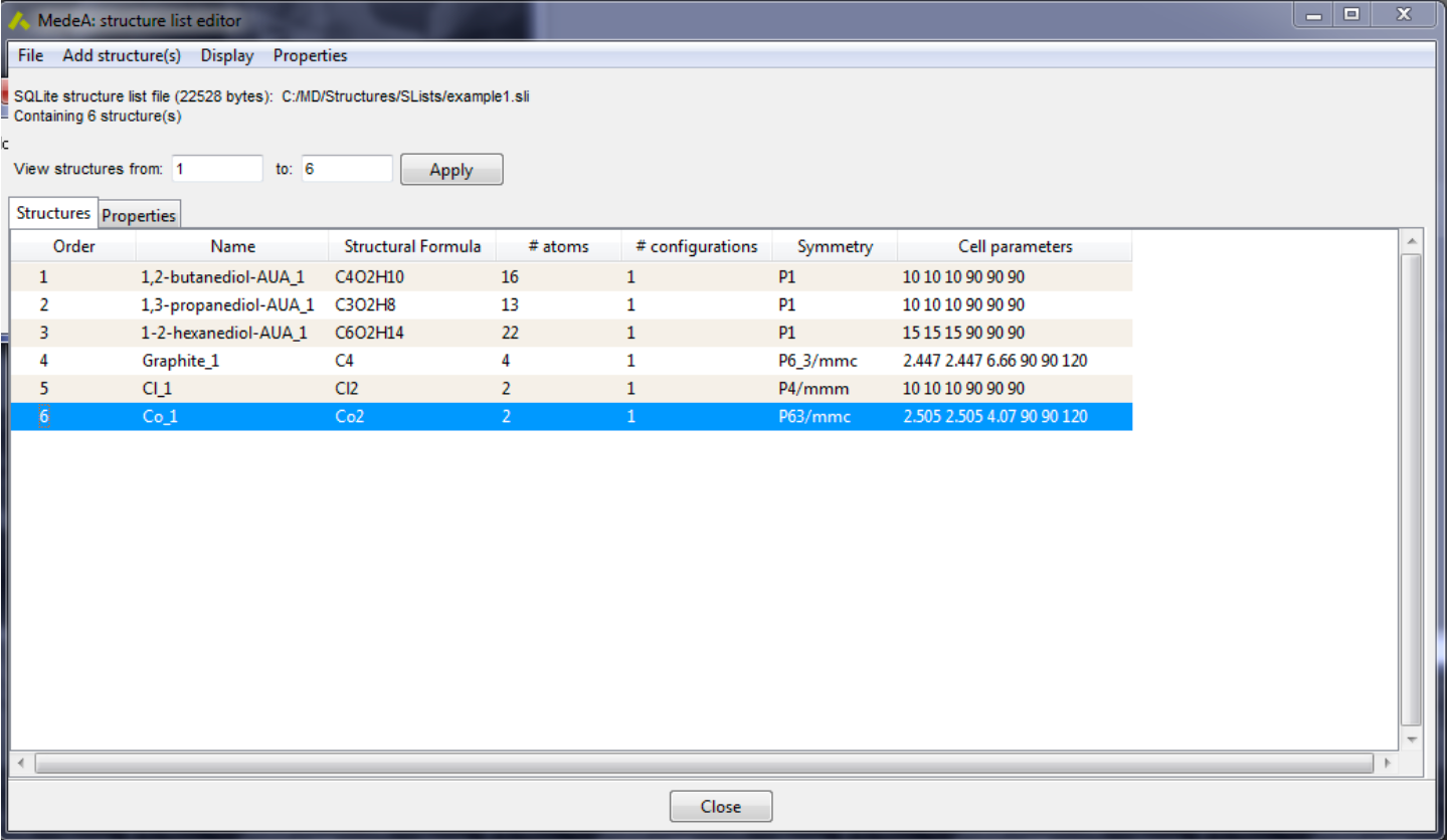
The descriptive part shows the file format, its size, and the full path. One can also control the number of displayed structures in the table, specifying the start and end index (clicking on the Apply button will update the view).
The Properties tab will show all properties in a table, as each structure can have its set defined, and as shown below the property:

2.32.3.3. File Formats
A Structure List has one of the following two formats:
- Text format: data is written in plain ASCII format. One can edit the content with a simple text file editor but with a high risk of erroneous modification. Many molecular dynamics jobs will produce a trajectory file in that format (Trajectory.dat or files with .traj extension). One cannot apply all available operations with that format.
- SQLite format: information is organized with an SQLite database format, which offers a much higher level of performance when processing and updating lists containing a large number of structures.
By default, the SQLite format is used when creating a new Structure List. It is recommended to convert to SQLite whenever possible, which can be done with the File >> Convert to SQLite/text format. It will create a file of the other type than the one displayed.
2.32.3.4. Add Structures
There are several ways to add structures to the current Structure List and they are accessible from the Add structures menu:

The different new structures sources are:
From MedeA:: invokes a dialog to select opened structures in the MedeA main window.
From files: opens a window to select individual structure files.
From a SMILES list file: selects an ASCII file (default .smi extension) formatted with two columns: the first for a molecule name and the second with the SMILES code.
Structure list from disk: select another Structure List from disk and add all its structures (with their properties) to the end of this one.
Structure list from job: select another Structure List from job and add all its structures (with their properties) to the end of this one.
Split structure(s) into molecule(s): selects a displayed structure in the MedeA main window and analyzes it different molecules (defined by bond connectivity, bond orders, atom elements). An aperiodic structure will be added for each molecule type, and every image will be added as a configuration.
Split structure(s) into molecule(s) with PBC: will do the same but with PBC.
2.32.3.5. Display
The information appearing in the structure table can be controlled by the Display menu selectors. The columns Order and Name will always be displayed.

The information displayed can be the structural information (Structural Formula, #atoms: number of atoms, #configurations: number of configurations, Symmetry and Cell parameters when in PBC) or user-defined properties. If a large number of properties is defined, only the first three will be displayed by default, others have to be selected from the Display menu to appear.
In case there are several configurations for a structure, the value shown in the table will correspond to the first configuration. Other configurations’ property values can be seen by choosing to show the structure properties in the Properties table.
2.32.3.6. Ordering and Numbering Structures
Structures are stored in a given order in the list, which appears in the Order column in the structures table. It is possible to change the order in the table by sorting rows (structures) according to a column from the right-click popup menu commands Sort Ascending or Sort Descending, on a column title. Also, a given structure can be moved up or down by a right-click on its row with the corresponding command in the popup menu.
If the initial order of the rows in the table is changed by one of these methods, the actual structure order in the Structure List file remains unchanged. It is possible to apply the new displayed order to reorder the list internal ordering with the right-click popup menu command Save the order of the rows. This can be useful, for example, to change the processing order in a job.
2.32.4. Delete Existing Properties
The Properties >> Delete menu command brings up a small dialog window summarizing the list of all existing properties for all structures. They can be selected for being deleted. Once the OK button is used the data is deleted and the file is updated, i.e. the deleted data is no more recoverable.

2.32.5. Create a New Property
The Properties >> New Property opens a small dialog window allowing to add a property to all current structures in the list. One has to provide the following:

Name: the property name
Units (optional): units that can apply to this property
Type: has to be one real (default), integer, or string
Size: the number of values for this property, default: 1
Dimension: the values dimension, e.g. ‘3 3’ would mean a 3 by 3 matrix
Default (optional): default value that will be added to all structures initially.
2.32.6. Edit Property Values
Values in user-defined properties can be interactively modified in several ways:
Double click on the displayed value turns it in editing mode. Pressing the ESC key will dismiss the change, OK will confirm it. If there are several configurations for a given structure, this action will update the value of the first configuration.
Copy, for example, values from a column in a spreadsheet and paste them in the target property column, using the right-click menu command Paste in <property>. Values will be added down starting from the row where the click was performed. This will update values for the first configuration in the updated structures.
Call the value editor from the right-click popup menu Edit <property> value. Each configuration value can be edited (changing configuration value can be done with a selector). Changes are applied only once the OK button is used. Of course, this is mostly useful if the structure has more than one configuration.

2.32.6.1. Copy property values
When default copy shortcut (usually Ctrl+/C) is pressed, and some rows are selected in the structure table, the content of the selected rows is copied to the clipboard and can later be pasted in e.g. an external spreadsheet. If some structures have more than one configuration, additional values corresponding to these additional configurations will not be included in the clipboard. Columns can be copied individually, using the right-click popup menu on a column title, as shown:

Either the full column can be copied to clipboard or the only values in selected rows.
2.32.6.2. Export Structures
Structures can be exported to individual structure files from the right-click popup menu:
- Individually to an individual structure file (.sci extension) with the Export structure<number> command, the <number> corresponding to the structure number in the row the click is made.
- All structures at once to individual structure files (.sci extension) with the Export all structures command. A filename prefix is used and the structure number and configuration (if more than one) are used for the final file name.
- All structures at once to the MaterialsDesign database with the Save All structure(s) to MD database command.
2.32.7. HT-Launchpad
The HT-Launchpad enables the automatic computation of materials properties for large sets of systems given in a Structure List. The two central items for this capability are (i) the Flowchart stage “ForEach Structure” and (ii) the Structure Lists described above.

The Flowchart stage ForEach Structure is conceptually simple yet extremely powerful. A file containing a Structure List is selected and by opening the Flowchart tab the various computational steps are specified in the form of a Flowchart which may contain stages running VASP, Gaussian, MOPAC, LAMMPS, and other steps. The results are added to the existing or new Structure Lists.
A checkbox enables parallel execution of the loop iterations, i.e. performing calculations on simultaneously on a sub-set of structures. The level of parallel execution is controlled by specifying the maximum number of jobs running simultaneously.
By checking the box “Advanced settings”, it is possible to skip structures in the loop over structures and to include loops over multiple configurations of a single structure, as shown below.

To add computed properties to a Structure List, the desired item is specified in a dialog box as shown below.

The name in the column “Source” has a specific format such as $Eelectronic_calc. A list of these properties is given in this User’s Guide in the chapter of MedeA Flowcharts.
The result of such a high-throughput calculation is stored in a Structure List as shown in the example below.

2.32.8. HT-Descriptors
The HT-Descriptor component of MedeA HT enables the definition and evaluation of descriptors. For example, if one is interested in the VASP energy per atom for the compounds given in the previous Structure List, one can define a descriptor which is simply the total energy computed with VASP divided by the total number of atoms.
To this end, open the Structure List with the computed VASP energies and select “Descriptors” from the pull-down menu “Properties”.

A dialog box will appear which allows the definition and the evaluation of descriptor. In the present example, the descriptor is called “eatom” and is defined as follows.

Application of this descriptor to the Structure List with the VASP energies results in a new column with the desired values. The display of this and all other columns can be controlled by selecting the corresponding item in the pull-down menu under “Display”.

In this example, the list is sorted by increasing energies per atom, which is accomplished by a right-click on the header of the column “eatom” and selecting sorting by ascending values.
After this simple example, the following text describes the functionality of the HT-Descriptor in detail.
HT-Descriptors enable the user to assign properties and descriptors to each structure in a Structure List, thus allowing classification and ranking of structures. A descriptor can be defined, for example, as a function of computed properties like elastic coefficients and topological properties such as the existence of channels in a structure. Sets of descriptors can be stored in catalogs, reloaded, and applied to newly created structure lists. Thus, Descriptors together with Structure Lists are a powerful tool in the context of high-throughput calculations.
Descriptors computed with this tool are scalar properties that can be defined as functional, using a set of mathematical operators and variables. They can be computed on the fly or submitted to a Flowchart. Values will be computed for every configuration of every structure when applicable.
A catalog is a collection of properties that are jointly defined. This notion is important since properties can be interdependent. They can be saved and loaded from files for later reuse, using buttons Load Catalog and Save Catalog. The Clear button will delete all existing descriptor definition data from this dialog.
The computation can be performed either interactively within MedeA by editing the Structure List or within a Compute descriptors List stage in a flowchart, which can be succeeding a stage used to create a Structure List, or simply to facilitate processing a large Structure List in a time-efficient manner.
2.32.8.1. Defining a descriptor
When the side button New is pressed, the dialog is configured to define a new descriptor. The following elements need to be provided:
- Name: It must obey the following rules: contain only lower case letters, numbers and the ‘_’ character. The first character has to be a lower-case letter
- Expression: The actual descriptor as a mathematical expression. One can directly type the expression or use the drop-down menu buttons to insert functions or structural data as a variable. The syntax rules are explained later
- Description: A describing text that will be saved in the catalog file, if the catalog is saved. The purpose is to allow the descriptor’s author to provide explanations to any other user that could use the catalog file.
Pressing the OK button below the Description will register the descriptor in the catalog and, it will appear in the catalog box. As property names in Structure Lists are not restricted to lower cases and allow other characters, one may wish to give a more detailed name for the property using the Assigned property column. One can edit it by double-clicking on it and type Enter to validate the new name, or Escape to dismiss it.
2.32.8.1.1. Syntax Rules
A descriptor’s expression obeys arithmetical edition rules: balanced parentheses, operands, and operators properly defined and ordered. The expression has to comply with the following syntax rules:
- Functions have to contain only upper-case letters and the ‘_’ character. All accessible functions can be inserted at the cursor position with the drop-down button menus related to functions. Arguments are enclosed within parentheses and separated by commas if more than one argument is needed. The opening parentheses must follow immediately after the last function character, e.g. POWER(a,3.0)
- Mathematical Operators: the + - / * signs are recognized. The power operator is accessible by the POWER(,) function. The AND or && (Boolean AND) and OR or // (Boolean OR) are also recognized in Boolean conditions when applicable.
- Operands can be an integer or real numbers or property names. Property names can contain only lower-case letters, numbers, and the ‘_’ character. Different types of properties can be used, and the drop-down menu button allows you to access by category. Some properties have a unit, and in that case, the default unit is mentioned in the list. If one wishes to use different compatible units, it has to be enclosed in parentheses right after the property name, e.g. volume(m^3). The property value will be automatically converted to the provided units.
- Expression elements have to be separated by spaces.

Clicking on a descriptor in the display list will display its name, its expression, and comments. A descriptor can be deleted by clicking the Delete button, or edited (change its name, expression or comments) with the Edit button.
In interactive mode, pressing the Compute button will start the computation of all descriptors in the catalog. When applicable the values will be stored in the list under the assigned properties. If the latter is not alcreated defined for a structure, it will be automatically created. If it alcreated exists, the content will be updated with newly computed values. If for some structures in the list, the descriptor cannot be computed, no value will be evaluated and the corresponding property will be left empty. For example, if a descriptor relies on the cell volume, it will not be computed for non-periodic structures in the present list.
2.32.8.2. Functions
Functions are of different categories, each corresponding to a drop-down menu button. They are recognized as upper case character strings.
2.32.8.2.1. Generic Mathematical Functions
Name Definition
ABS() Returns the absolute value
ACOS() Returns the arc cosine
ASIN() Returns the arc sine
ATAN() Returns the arc tangent
ATAN2() Returns the arc tangent of the two arguments
CEILING() Returns the smallest integer value not less than the argument
COS() Returns the cosine
COT() Returns the cotangent
DEGREES() Convert radians to degrees
EXP() Exponential of
FLOOR() Returns the largest integer value not greater than the argument
LOG() Returns the natural logarithm of the first argument
LOG10() Returns the base-10 logarithm of the argument
PI() Returns the value of pi
POWER() Returns the argument raised to the specified power
RADIANS() Returns argument converted to radians
ROUND() Round the argument
SIGN() Returns the sign of the argument
SIN() Returns the sine of the argument
SQRT() Returns the square root of the argument
TAN() Returns the tangent of the argument
2.32.8.3. Variables
Function operands can be either actual numbers or variables referring to structure properties. Atomic properties are defined for most per-element tabulated properties. Atomic properties related to nearest neighbors or ligands are specific, and if they appear in the descriptor definition they will trigger the computation of nearest neighbors for that structure. By definition, the ligands and voids properties and function will also trigger that computation.
2.32.8.3.1. Recursive Definition
Within the same catalog, one can refer to another descriptor directly by its name. The recursive dependency will be detected, and the computation order will follow it. Of course, cycling dependencies will cause an error.
2.32.8.3.2. Existing Descriptors
Properties alcreated defined in the list can be used as variables to define new descriptors. Only scalar numerical properties can be understood as existing descriptors. To refer to existing descriptors, the @ is used, and apart from that, the syntax should still be lower case letters and numbers. For this reason, an automatic mapping from existing property names is done by lowering letter case and removing other characters, e.g. “Exp. Density” should be referred to as @expdensity.
2.32.8.4. Coordination properties
Whenever a property or a function related to ligands (nearest neighbors) is included in one of the catalog descriptors expression, a quick search for nearest neighbors will be triggered. This neighbor analysis comprises two steps:
- Firstly, all neighboring atoms that are not Voronoi neighbors are excluded. Voronoi cells are defined around each atom, as the portion of space where each point is closer to that atom than any other. Atomic extents are defined by atomic radii, and this Voronoi analysis provides a superior criterion for neighbor selection when a structure contains species with differing atomic radii. (Because if the segment from a particular atom to a neighboring atom intersects the Voronoi cell of a third atom, that potential neighbor can be discarded).
- Secondly, reduced distances between an atom and its neighbors are computed as the distance divided by the sum of atomic radii. The largest gap in the neighbor’s reduced distances distribution is considered to separate nearest neighbors from further neighbors, and this criterion is employed to detect nearest neighbors.
As mentioned, covalent atomic radii are the default. However, it is also possible to use an alternative list of radii that is composed of covalent radii for elements found mostly in neutral condition and ionic radii that are the most frequent for atoms elements like Li. For simplification, this alternative list is labeled as Ionic (the default is labeled Covalent) and can be selected before actually computing descriptors where coordination comes into play.

Once the coordinated neighbors have been computed, the coordinated geometry class can be computed. To that end, both the distance to neighbors and the angles between each vector joining the atoms to its coordinated neighbors are analyzed. As in many cases, there will not be an exact match in distances and angles to a given regular coordination geometry, two additional values are also computed, namely
Distance dispersion the maximum distance deviation from the average neighbor distances.

Angular dispersion the maximum angle deviation from all the ideal case angles.

As a result, each atom of each structure is characterized by the following:
- coordination (no units): the coordination number.
- coordination_confidence (no units): the coordination confidence score. In some cases, the systematic discrimination of neighboring atoms as the ligand is not unquestionable: some neighboring atoms might or might not be ligands. This confidence score accounts for this uncertainty: its lower limit is 0 meaning no confidence and 1 means that the coordination number is established.
- coordination_class (no units): the coordination class geometry code (a string representation can be used instead of the integer code), see the coordination class table.
- coordination_ddispersion (no units): coordination distance deviation mentioned above.
- coordination_adeviation (degrees): angular deviation
The coordination class values can be inserted in the expression editor with the Coordination class drop-down menu button.
2.32.8.5. Voids Properties
Voids are characteristics of voids topology: empty spaces such as cages, layers, or tunnels. Whenever a property or a function related to voids is included in the catalog descriptors expression, a quick search for voids is triggered. The search algorithm for the voids analysis is based on a multi-scale cell subdivision. The idea is to approximate the void space with void subcells up to a given precision. In the case of a cubic cell, these subcells are cubes. According to this analysis, connected sets of void subcells (subcells that are entirely included in void space) are identified as voids volume. They are characterized by:
- void volume (Ang^3): the sum of the void subcell volume.
- cage diameter (Ang): the diameter of the largest sphere that could stand in the void.
This estimation is based on the subcells sizes decomposition and should be understood as a lower limit. A finer analysis would provide an actual higher estimate in most cases.
- cross diameter (Ang): the diameter of the largest sphere that could diffuse through the void, using the periodic conditions of the cell. This estimation is based on the subcells sizes decomposition and should be understood as a lower limit. A finer analysis would provide an actual higher estimate in most cases.
As these properties rely on approximation, an inherent uncertainty value is available for each of these diameters, labeled e.g. delta_cage_diameter. These properties can be inserted with the Voids properties drop-down button. Each structure may have any number of voids, each belonging to one of these 3 classes:
- 0: cage closed void, no diffusion is possible. The cross diameter is 0 Ang.
- 1: channel there is at least one crossing path in the void. The cross diameter is higher than 0.
- 2: layer the void divides the cell space in 2 distinct parts (except the void itself).
These class numbers correspond to the void_class property.
2.32.8.6. Examples
2.32.8.6.1. Mass Density
It can be defined as:
Mass_density=SUM_ATOM(atomic_mass(Mg))/volume(m^3)
Let’s say we want to compute the density of materials in the case all hydrogen atoms are removed. It can be achieved by taking into consideration all the atoms of the unit cells that are not hydrogen i.e. which atomic number is greater than 1. That’s what we call Not H density with descriptor name not_h_density and its definition is using a filtering criterion ( atomic_number>1):
not_h_density=MATCH_ATOM_SUM(atomic_number>1,atomic_mass(Mg))/volume(m^3)
Now, to illustrate how computed properties can be recursively defined, let us define the ratio of in-cell hydrogen mass density over total mass density, that we name H density ratio with the following definition:
h_density_ratio=(mdensity-not_h_density)/mdensity
2.32.8.6.2. Coordination
To illustrate the coordination geometry, we focus on C atoms in tetrahedral coordination. We will also pay attention to the deviation (in angle and distance) from the exact tetrahedral conformation. To this end, we define these 3 properties.
Tetrahedral C: the count of C atoms in tetrahedral conformation: tetrac=MATCH_ATOM_SUM(atomic_number=6 && coordination_class=COORD_4_TETRAHEDRAL,1)
Tetrahedral C angle deviation: The maximum tetrahedral C angle deviation tetrac_adev=MATCH_ATOM_MAX(atomic_number=6 && coordination_class=COORD_4_TETRAHEDRAL, coordination_adeviation)
Tetrahedral C distance dispersion: The maximum tetrahedral C distance dispersion tetrac_ddev=MATCH_ATOM_MAX(atomic_number=6 && coordination_class=COORD_4_TETRAHEDRAL,coordination_ddispersion)
Note that the filtering condition are using &&, the logical AND operator, and that a coordination constant has been used (the 440 value could have been used instead).
2.32.8.6.3. Ligands
Here are some properties related to atom-ligand properties. First the average atom-ligand distance, that defined as a double average, first level on all atoms, second level on all ligands (for each atom):
Avgdistligand=AVG_ATOM(AVG_LIGAND ligand_distance(Ang)))
Then the average number of ligands per atom:
avgnligand=AVG_ATOM(SUM_LIGAND(1))
Finally, the average atom_ligand atom, excluding the hydrogens (as atom and as ligand), which implies 2 filtering average functions:
avgdistligand_not_h=MATCH_ATOM_AVG(atomic_number>1, MATCH_LIGAND_AVG(ligand_atomic_number>1,ligand_distance(Ang)))
2.32.8.6.4. Voids
Here is a list of simple descriptors for voids:
caged (void cage diameter): The maximum (of any void) cage diameter: MAX_VOID(cage_diameter(Ang))
crossd (void cross diameter): The maximum (of any voids) cross diameter: MAX_VOID(cross_diameter(Ang))
ncages (number of cages): The number of cages in the system: MATCH_VOID_SUM(void_class=0,1)
nchannels (number of channels): The number of distinct channels in the system: MATCH_VOID_SUM(void_class=1,1)
nlayers (number of layers): The number of distinct layers in the system: MATCH_VOID_SUM(void_class=2,1)
nvoids nNumber of voids): The number of distinct voids in the structure: SUM_VOID(1)
voidv (void volume ratio): The void volume over total volume ratio: SUM_VOID(void_volume)/volume
2.32.8.7. MPM
The description above refers to operations on a Structure List. MedeA HT also offers the ability to create descriptors operating on entire crystallographic structural databases available in MedeA InfoMaticA, i.e. on hundreds of thousands of structural entries. This is called Materials Property Mining (MPM). While operations on Structure Lists are dynamic and can involve newly computed properties such as DFT total energies or elastic coefficients, MPM is designed to work with pre-computed properties such as coordination numbers and voids. The properties available within MPM are computed in advance and delivered with the databases.
Analogous to the definition of descriptors illustrated above, MPM allows the construction of descriptors which then can be applied to all entries in the InfoMaticA databases containing the relevant structural information (i.e. atomic positions in stoichiometric compounds). Thus, MPM is an extremely powerful data mining tool, which can be used in conjunction with the descriptors operating on Structure Lists.
| download: | pdf |
|---|